Quantitative Edge: Building Algorithmic Forex Strategies with Python
A masterclass in transforming technical analysis into automated execution systems.
The foreign exchange market operates as a relentless stream of data, characterized by high-frequency fluctuations and vast liquidity. For the discretionary trader, processing this volume of information manually introduces cognitive fatigue and emotional bias. Algorithmic trading solves this by codifying technical analysis into a systematic, rule-based framework. Python has emerged as the industry standard for this transition, offering a balance of readability and high-performance libraries that allow traders to build, test, and deploy sophisticated models with institutional precision.
The Professional Python Stack
Success in quantitative finance requires the right infrastructure. Python’s ecosystem provides specialized tools for every stage of the pipeline, from data ingestion to mathematical optimization. A professional algo-trading environment typically centers around a core set of libraries designed to handle time-series data efficiently.
| Library | Core Functionality | Role in the Pipeline |
|---|---|---|
| Pandas | Data Manipulation & DataFrames | Storing and cleaning time-series price data. |
| NumPy | Numerical Computing | Performing high-speed vectorized calculations. |
| Pandas_TA | Technical Analysis Indicators | Calculating RSI, MACD, and Bollinger Bands. |
| Matplotlib | Data Visualization | Plotting equity curves and drawdowns. |
| SciPy | Scientific Computing | Optimizing parameters via regression or solvers. |
Data Acquisition and Vectorization
The first hurdle is obtaining clean, high-granularity data. Most algorithms operate on OHLCV (Open, High, Low, Close, Volume) data. In Python, we treat this data not as a sequence of individual points, but as a "Vector." Vectorization allows us to apply mathematical operations across an entire dataset simultaneously, rather than using slow loops. This is essential for backtesting strategies across years of 1-minute data in seconds.
import pandas as pd
import numpy as np
df['SMA_50'] = df['Close'].rolling(window=50).mean()
df['SMA_200'] = df['Close'].rolling(window=200).mean()
# Generating Signals without Loops
df['Signal'] = np.where(df['SMA_50'] > df['SMA_200'], 1, 0)
df['Position'] = df['Signal'].diff()
Architecting a Technical Strategy
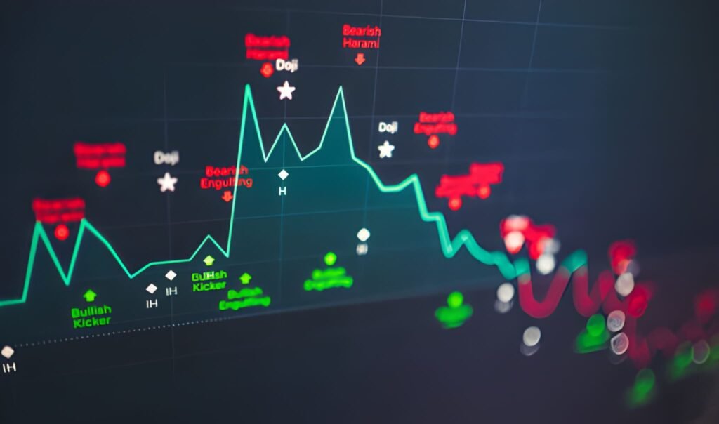
A technical strategy in an algorithmic context must be binary: it is either "True" or "False." Ambiguity is the enemy of automation. Most developers start with trend-following or mean-reversion frameworks. For instance, a "Dual Moving Average Crossover" is a trend-following system that seeks to capture momentum when short-term price average exceeds long-term average.
Logic: Enters when momentum is confirmed. Uses indicators like SMA, EMA, or ADX. High win-rate in volatile, trending markets but suffers during consolidation.
Logic: Bets that price will return to a historical average. Uses RSI or Bollinger Bands. High win-rate in ranging markets but high risk during breakouts.
Vectorized vs. Event-Driven Testing
There are two primary ways to test your strategy. Vectorized Backtesting is fast and ideal for initial research. It calculates returns across the entire historical matrix at once. However, it ignores "execution reality" like slippage and spread. Event-Driven Backtesting simulates every tick or bar sequentially, replicating the logic of a live exchange. While slower, it is the only way to verify how an algorithm will behave during periods of low liquidity or sudden price gaps.
The Math of Quantitative Risk
The most important part of your Python script is not the entry signal, but the risk management module. A professional algorithm must calculate its own "Position Size" based on current volatility and account equity. We use the Average True Range (ATR) to determine where a stop-loss should sit and then work backward to define the lot size.
Equity: $100,000
Risk per Trade: 1.0% ($1,000)
ATR (14-period): 0.0020 (20 pips)
Stop Loss Multiplier: 2.0x ATR (40 pips)
Position Size Calculation:
Units = Risk Amount / (Stop Loss in Pips * Pip Value)
Units = $1,000 / (40 * $10 for Standard Lot)
Units = 2.5 Standard Lots
The Sharpe Ratio measures the performance of an investment compared to a risk-free asset, after adjusting for its risk. In Python, we calculate this by dividing the average excess return by the standard deviation of returns. A Sharpe Ratio above 1.0 is considered good, while above 2.0 is exceptional for an automated system.
Max Drawdown is the largest peak-to-trough decline in an account's equity curve before a new peak is attained. An algorithm might have high returns, but if it has a 50% MDD, it is likely to cause a complete account wipeout during a black swan event. Systematic traders prioritize low MDD over high absolute returns.
API Connectivity and Execution
Once a strategy passes the backtest, it must connect to a brokerage API. Professional traders often use Interactive Brokers (ib_insync) or OANDA for foreign exchange. The Python script enters a "Live Loop," where it fetches the latest market data every minute, calculates indicators, checks if entry conditions are met, and sends a "Market Order" or "Limit Order" if a signal is triggered.
Live trading requires high-uptime infrastructure. Most professionals do not run their Python scripts on home computers. Instead, they utilize Virtual Private Servers (VPS) located in data centers near the exchange servers (e.g., in London or New York) to minimize latency and ensure the script runs 24/7 without interruption from power outages or local internet failures.
Dealing with Overfitting
The biggest threat to an algorithmic trader is Overfitting. This occurs when you tune your parameters (e.g., changing an SMA from 50 to 47.5) to perfectly fit historical data. While the backtest looks flawless, the strategy will fail in live markets because it has memorized "noise" rather than "signal." To combat this, quantitative analysts use Walk-Forward Analysis and Monte Carlo Simulations to stress-test the robustness of their logic.
Transitioning to algorithmic trading with Python is a significant evolution for any investor. It requires a shift from "chart reading" to "system engineering." By combining the analytical power of Pandas, the speed of NumPy, and a rigorous approach to risk management, you can build a trading engine that operates with the cold, calculated efficiency of an institutional desk. The market is unpredictable, but your reaction to it through code can be perfectly disciplined.